In this article we will learn how to test for normality in R using various statistical tests.
Theory
In statistics, it is crucial to check for normality when working with parametric tests because the validity of the result depends on the fact that you were working with a normal distribution.
Therefore, if you ran a parametric test on a distribution that wasn’t normal, you will get results that are fundamentally incorrect since you violate the underlying assumption of normality.
Of course there is a way around it, and several parametric tests have a substitute nonparametric (distribution free) test that you can apply to non normal distributions.
For the purposes of this article we will focus on testing for normality of the distribution in R.
Namely, we will work with weekly returns on Microsoft Corp. (NASDAQ: MSFT) stock quote for the year of 2018 and determine if the returns follow a normal distribution.
Application
Below are the steps we are going to take to make sure we master the skill of testing for normality in R:
- Importing 53 weekly returns for Microsoft Corp. stock
- Calculating returns in R
- Plotting returns in R
- Kolmogorov-Smirnov test in R
- Shapiro-Wilk test in R
- Jarque-Bera test in R
Part 1. Importing 53 weekly returns for Microsoft Corp. stock
In this article I will be working with weekly historical data on Microsoft Corp. stock for the period between 01/01/2018 to 31/12/2018.
The data is downloadable in .csv format from Yahoo! Finance.
After you downloaded the dataset, let’s go ahead and import the .csv file into R:
mydata<-read.csv("/Users/DataSharkie/Desktop/MSFT.csv", header=TRUE)
Now, you can take a look at the imported file:
View(mydata)
The file contains data on stock prices for 53 weeks. The first issue we face here is that we see the prices but not the returns. We will need to calculate those!
Part 2. Calculating returns in R
To calculate the returns I will use the closing stock price on that date which is stored in the column "Close".
Let's store it as a separate variable (it will ease up the data wrangling process).
One approach is to select a column from a dataframe using select() command. But her we need a list of numbers from that column, so the procedure is a little different.
Let's call our new vector "x".
Let's get the numbers we need using the following command:
x<-mydata$Close
The reason why we need a vector is because we will process it through a function in order to calculate weekly returns on the stock.
The formula that does it may seem a little complicated at first, but I will explain in detail.
Run the following command to get the returns we are looking for:
x<-as.data.frame(diff(x)/x[-length(x)])
The "as.data.frame" component ensures that we store the output in a data frame (which will be needed for the normality test in R).
The "diff(x)" component creates a vector of lagged differences of the observations that are processed through it.
The last component "x[-length(x)]" removes the last observation in the vector. Why do we do it? Since we have 53 observations, the formula will need a 54th observation to find the lagged difference for the 53rd observation. We don't have it, so we drop the last observation.
The last step in data preparation is to create a name for the column with returns. It will be very useful in the following sections.
Let's name the returns column "r".
You can add a name to a column using the following command:
names(x)<-"r"
Part 3. Plotting returns in R
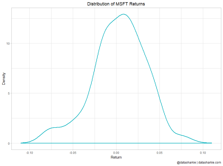
After we prepared all the data, it's always a good practice to plot it.
The distribution of Microsoft returns we calculated will look like this:
Part 4. Kolmogorov-Smirnov test in R
One of the most frequently used tests for normality in statistics is the Kolmogorov-Smirnov test (or K-S test).
In this tutorial we will use a one-sample Kolmogorov-Smirnov test (or one-sample K-S test). It compares the observed distribution with a theoretically specified distribution that you choose.
This is a quite complex statement, so let's break it down.
In this tutorial, we want to test for normality in R, therefore the theoretical distribution we will be comparing our data to is normal distribution.
It is important that this distribution has identical descriptive statistics as the distribution that we are are comparing it to (specifically mean and standard deviation.
The null hypothesis of the K-S test is that the distribution is normal.
Therefore, if p-value of the test is >0.05, we do not reject the null hypothesis and conclude that the distribution in question is not statistically different from a normal distribution.
For K-S test R has a built in command ks.test(), which you can read about in detail here.
We are going to run the following command to do the K-S test:
ks.test(x$r, "pnorm", mean=mean(x$r), sd=sd(x$r))
We should get the following output:

The p-value = 0.8992 is a lot larger than 0.05, therefore we conclude that the distribution of the Microsoft weekly returns (for 2018) is not significantly different from normal distribution.
Part 5. Shapiro-Wilk test in R
Another widely used test for normality in statistics is the Shapiro-Wilk test (or S-W test).
The procedure behind the test is that it calculates a W statistic that a random sample of observations came from a normal distribution.
Similar to Kolmogorov-Smirnov test (or K-S test) it tests the null hypothesis is that the population is normally distributed.
The S-W test is used more often than the K-S as it has proved to have greater power when compared to the K-S test.
From the mathematical perspective, the statistics are calculated differently for these two tests, and the formula for S-W test doesn't need any additional specification, rather then the distribution you want to test for normality in R.
For S-W test R has a built in command shapiro.test(), which you can read about in detail here.
We are going to run the following command to do the S-W test:
shapiro.test(x$r)
We should get the following output:

The p-value = 0.4161 is a lot larger than 0.05, therefore we conclude that the distribution of the Microsoft weekly returns (for 2018) is not significantly different from normal distribution.
Part 6. Jarque-Bera test in R
The last test for normality in R that I will cover in this article is the Jarque-Bera test (or J-B test).
The procedure behind this test is quite different from K-S and S-W tests.
The J-B test focuses on the skewness and kurtosis of sample data and compares whether they match the skewness and kurtosis of normal distribution.
R doesn't have a built in command for J-B test, therefore we will need to install an additional package.
When it comes to normality tests in R, there are several packages that have commands for these tests and which produce the same results.
In this article I will use the tseries package that has the command for J-B test. You can read more about this package here.
Note: other packages that include similar commands are: fBasics, normtest, tsoutliers.
In order to install and "call" the package into your workspace, you should use the following code:
install.packages("tseries")
library(tseries)
The command we are going to use is jarque.bera.test().
Similar to S-W test command (shapiro.test()), jarque.bera.test() doesn't need any additional specifications rather than the dataset that you want to test for normality in R.
We are going to run the following command to do the J-B test:
jarque.bera.test(x$r)
We should get the following output:

The p-value = 0.3796 is a lot larger than 0.05, therefore we conclude that the skewness and kurtosis of the Microsoft weekly returns dataset (for 2018) is not significantly different from skewness and kurtosis of normal distribution.
I hope this article was useful to you and thorough in explanations. I encourage you to take a look at other articles on Statistics in R on my blog!